Modeling Axial Losses: Methods and Consequences

In 2D simulations, where the axial (parallel) direction is not explicitly modeled, axial ion losses can be represented statistically by removing ions with a prescribed probability. This approach approximates the effect of particles escaping along magnetic field lines to the end plates of the device.

In EDIPIC-2D, axial ion losses are implemented using a constant loss frequency, calculated based on the expected ion escape time. This frequency can be estimated using the Bohm velocity, which characterizes the ion outflow velocity at a sheath edge.

Bohm Velocity

Physically, the Bohm velocity is given by:

v_B = √(k_B T_e / m_i)

where T_e is the electron temperature and m_i is the ion mass. Assuming ions stream out along the axial direction at approximately v_B = 1×10⁴ m/s, the characteristic loss frequency can be estimated as:

f_loss ≈ v_B / L_Axial

where L_Axial is the effective axial length of the device or simulation domain, considered to be 10 cm. In the code, this frequency is translated into a probabilistic particle removal mechanism, as shown below:

Subroutine PERFORM AXIAL ION LOSS in EDIPIC-2D, implementing probabilistic ion removal based on a fixed loss rate.

Effect of Axial Loss Mechanism

The effect of this axial loss mechanism is illustrated below, showing a comparison of the total ion inventory over time for two cases: with and without axial ion loss.

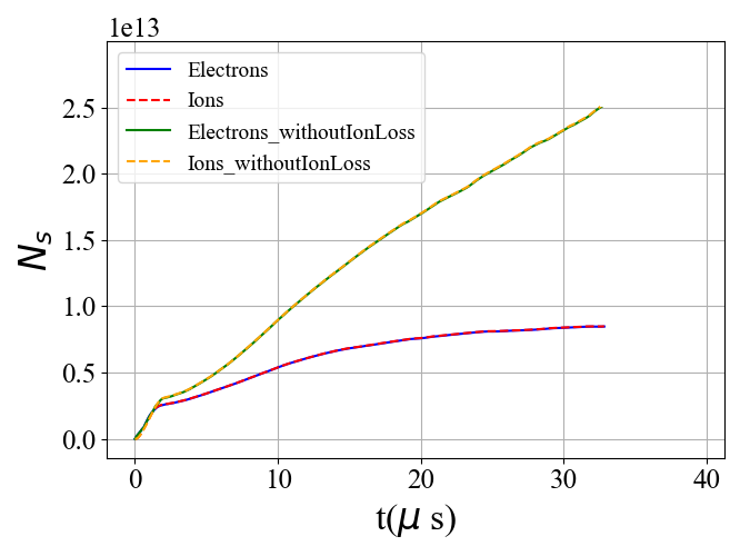
Time evolution of total electron and ion inventories in simulations with and without axial ion loss. Ion and electron inventories stabilize when axial loss is included, while they grow unphysically without the loss mechanism.